Overview
I've been playing with the ARC AGI Prize recently1. There are a lot of things that surprised me while replicating the approach of last year's grand prize winner, "The ARChitects"2. For example, when the model was less sure about a pixel, the solution was more likely wrong. Another was that a per-pixel token encoding even worked. It was like the poor model was forced to type its solutions out, character by character, on a typewriter with no backspace.
Imagine solving a jigsaw puzzle but you have to place pieces starting from the top-left corner in order. No jumping around. No doing the edges first. That's what we're making these models do.
Instead of forcing the model to work in typewriter-order, what if we let it fill in the easy parts first? Maybe you can use the uncertainty to measure what is obvious and what is tricky. As it turns out, it works:
Video 1: A comparison of autoregressive (left) and diffusion (right) approaches on the same task. The diffusion model first fills in "easy" tokens and works its way in to more complicated tokens.
Based on recent work in converting autoregressive LLMs into diffusion models3, I took my autoregressive model and hacked it to be able to decode in any order. Then I had it unmask tokens it was more confident about first. You can see more animated detail below in How Generation Works.
Skipping ahead a bit to the results: it still needs more work. My diffusion approach is faster at 10 timesteps and achieves modestly better token accuracy, but this doesn't translate into solving more tasks. At 30 timesteps - where it finally matches the baseline's task success rate - it's actually slower than autoregressive.
Why? One thing the typewriter approach has going for it is that the constraint of only moving forward makes it easy to cache. My implementation can't do this. I've converted the "decoder" style LLM into a single fully connected "encoder" style, where activations of previous tokens are allowed to change based on later tokens. Currently this makes the input tokens uncachable. However, I think changing the input activations based on output changes is more flexibility than ARC tasks need. I can get back caching of the input tokens with some tweaks to disable this, which I get into in the Next Steps section at the end.
This post chronicles my process in adapting a fine-tuned Qwen3-8B model4 for diffusion-based ARC solving, following recent work on converting language models to diffusion3. I crammed in a lot of detail, I recommend reading the process section and then skipping around.
Table of Contents
The Process: How diffusion decoding works on ARC tasks
What Do the Tasks Look Like? • How Generation Works • Why Better Pixel Accuracy Alone Doesn't Solve Puzzles
Background: Motivation and failed alternatives
The ARChitects Baseline • Computational Bottlenecks • Alternatives Considered • Diffusion Models Are Hard To Train From Scratch
Technical Implementation: Training details and code snippets
The Approach • Hyperparameters • Training Process • Batch Structure • Training Data and Augmentation • Handling Fixed Sequence Lengths
Results on ARC Prize 2025 Evaluation Set: Performance metrics and analysis
Overall Performance Comparison • Performance by Output Size • Task Success Rates • Results Analysis
Next Steps • Conclusion • Acknowledgments
The Process
What Do the Tasks Look Like?
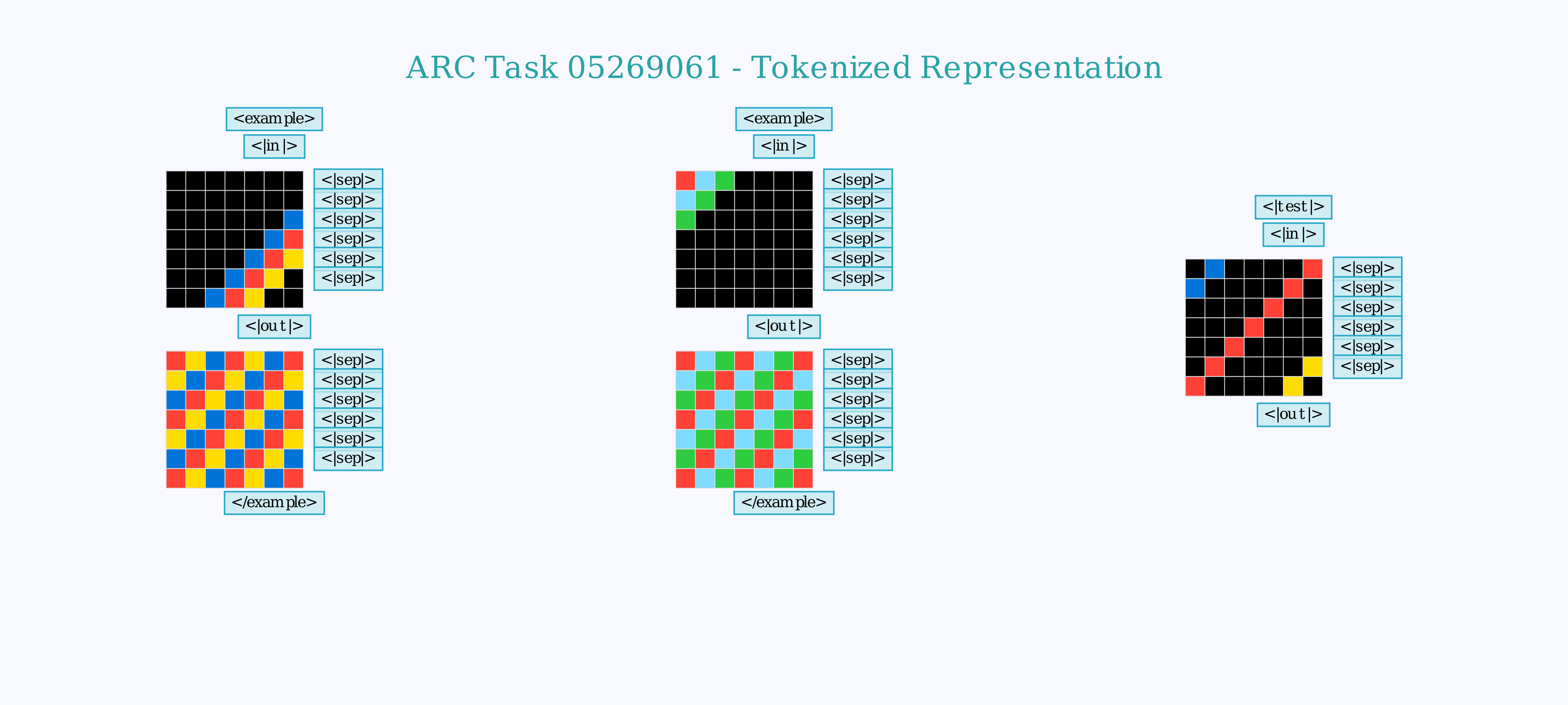
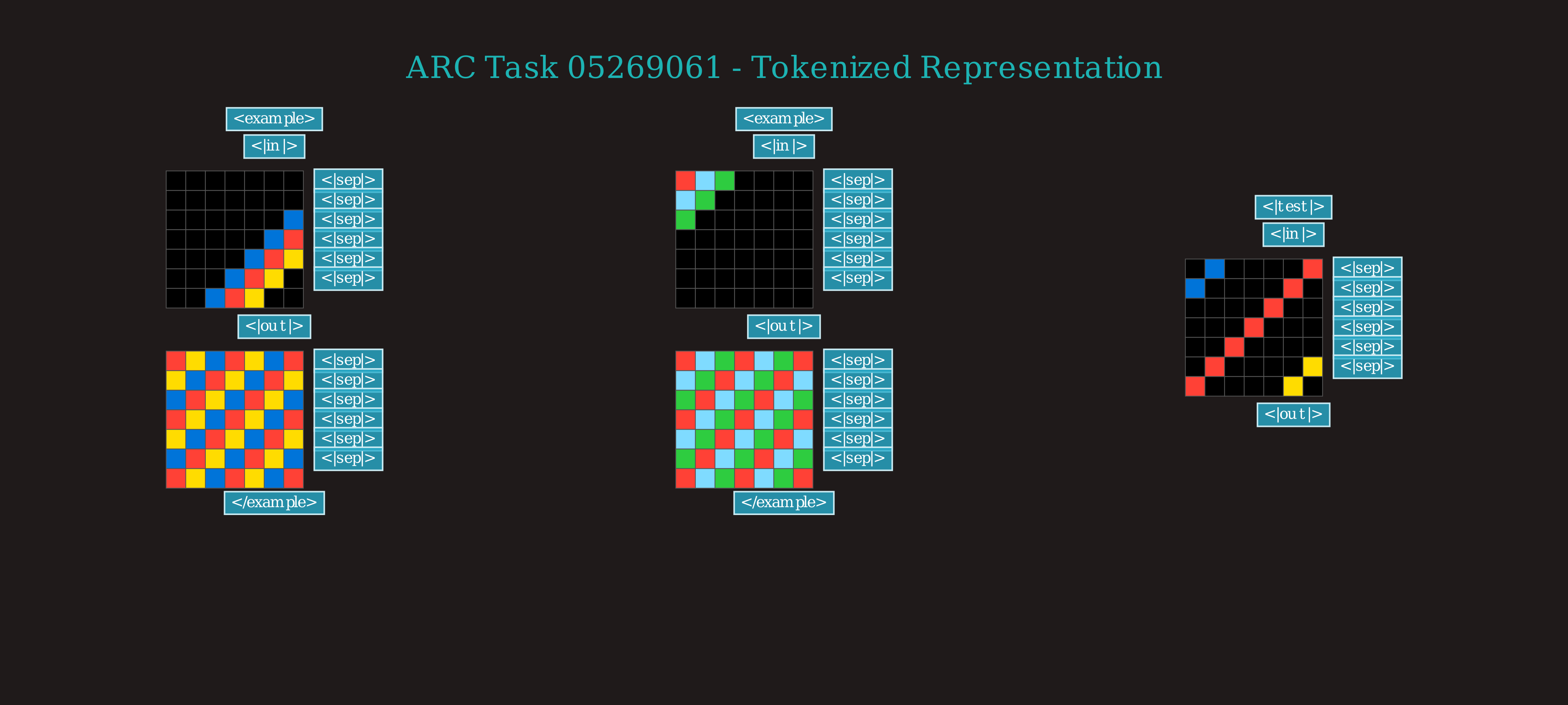
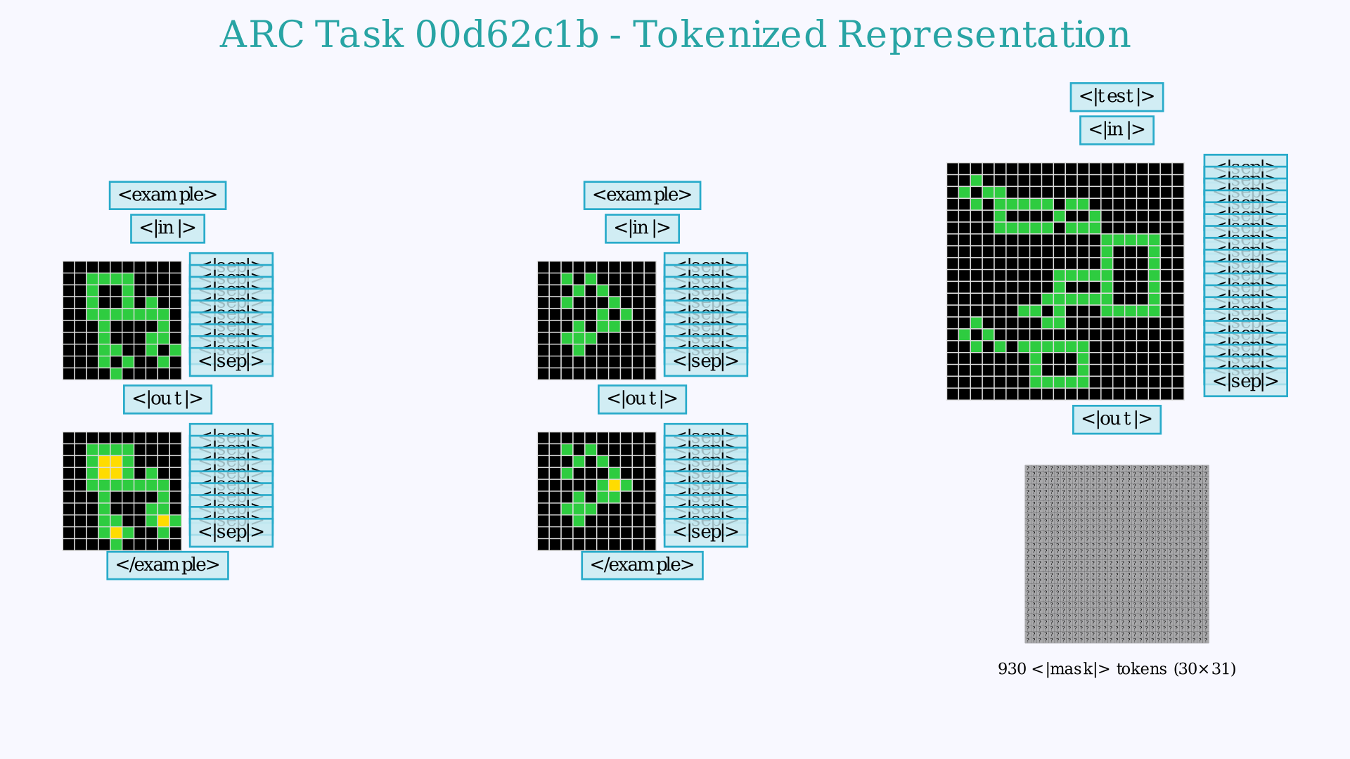
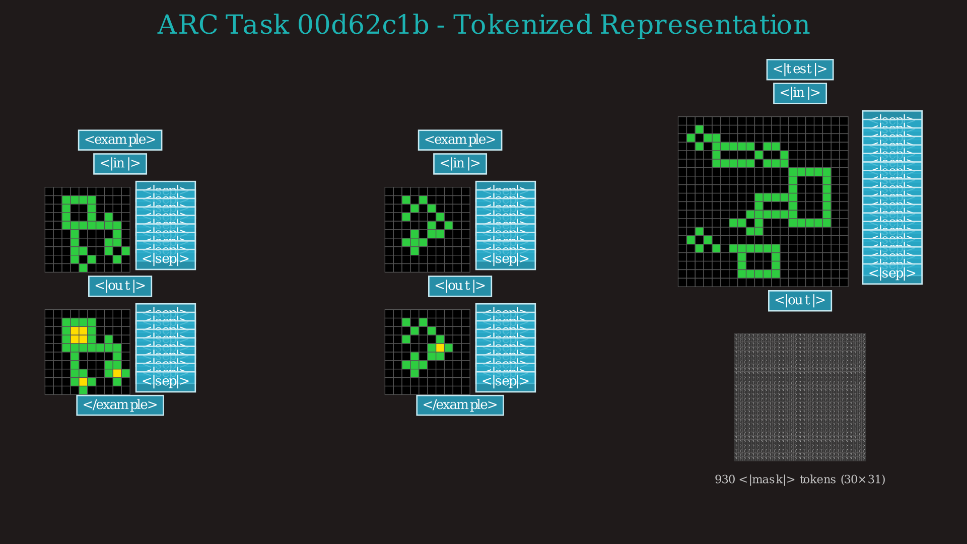
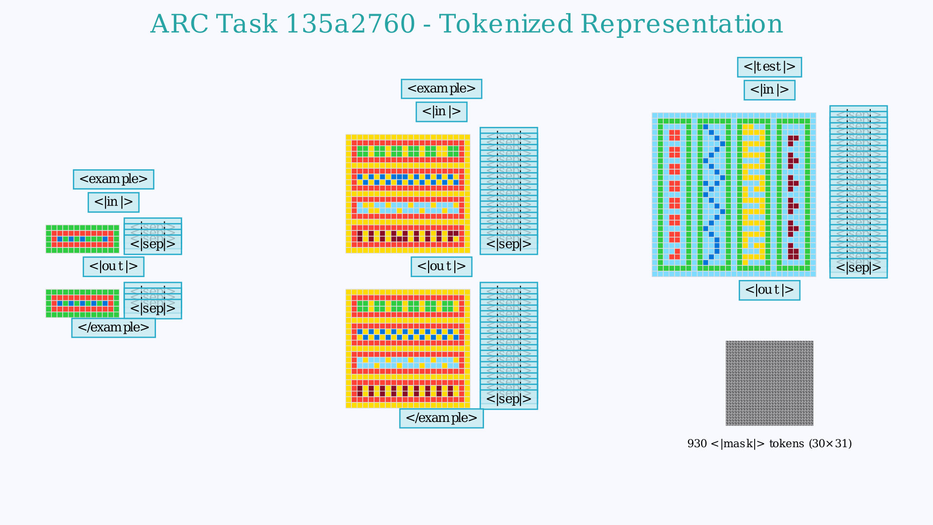
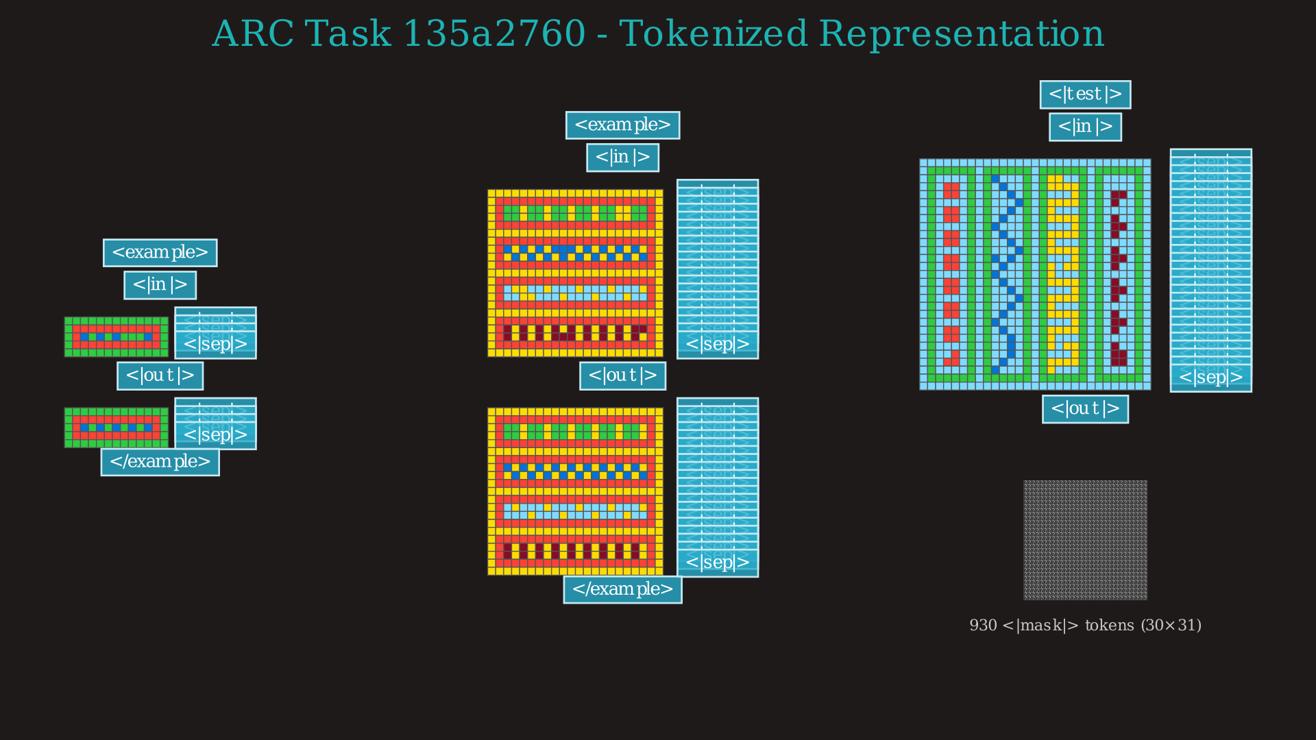
You can click to expand the images below to see the complete encoding grid. Note that while the videos focus only on the final test output for clarity, the model actually processes the entire context including multiple demonstration examples. The vocabulary of the model has been reduced to a set of 24 new tokens, representing each of the 10 numbers a grid cell can have as well as several "tags" that denote the structure of the grid or whether a grid is an input or an output, an example or the final test.
×
While I display it in grids in other visualizations, the model actually "sees" a 1D stream of tokens. This is the first part of that sequence, truncated right after the first input grid of the first example.


×


How Generation Works
As you can see in the comparison in the overview above, while the autoregressive model fills in tokens left-to-right, the diffusion model starts with tokens matching what the test input gives for the answer, then works its way into the harder tokens that require understanding the task to fill in correctly. The core idea is to start with a fully masked output grid and iteratively fill in the tokens the model is most confident about, regardless of their position.
In each step, the model:
1. Evaluates all masked positions
2. Ranks predictions by entropy (lower entropy = higher "confidence")5
3. Unmasks the most certain predictions
4. Repeats with the partially solved grid
Here's an animation of the whole process:
Video 2: Confidence-based diffusion process on a simple task from the training set. Note that the numbers in the visualization of this particular task are too close and all round to 1.0, but the color range has been tightened to show the differences.
In the example above, you can see it first fill in the shape of the pattern and cells that match the test input. In other cases, it selects the background tokens first, and then gradually gains confidence around the more complicated patterns:
Video 3: Qwen3-8b finetune with a Diffusion LoRA solving a more complex task.
×
This behavior is entirely emergent from choosing low entropy predictions - the model learned this without explicit supervision.
What worked well: Despite the accuracy-speed tradeoff, the diffusion approach successfully achieved non-sequential solving. For simple patterns, it can generate correct outputs in just 10 timesteps, and the emergent "easy-first" behavior shows the model learned meaningful confidence estimates without explicit supervision.
Why Better Pixel Accuracy Alone Doesn't Solve Puzzles
While diffusion achieves 3% higher token accuracy overall, this doesn't translate to more correctly solved tasks. Here's a revealing example task - even with higher average accuracy, the model still misses the underlying symmetrical patterns:
×
Video 4: An example of the model failing to solve a task from the evaluation set despite better average accuracy
Take this failure case - the model needs to recognize what the pattern should be, not just copy what it's seen. And as shown above, this isn't something solving the problem out of order really helps with.
Humans benefit from extensive pretraining on geometric patterns and symmetries that these models lack. The ARChitects' augmented re-ranking approach6 makes up for this by including the symmetries and invariants as part of the ranking process. When you rotate or reflect a candidate solution, correct patterns like this maintain their symmetry while errors create obvious asymmetries. This technique improved their accuracy by ~25%.
The diffusion LoRA does not translate into additional completely solved tasks on its own. The hope is: diffusion speeds up generation → more time for generating candidates to rank → exploit augmentation to catch errors during ranking → better generalization.
Background
I detail below a bit more about the motivations of why this might be useful, how I got it working, and where it still falls short.
The ARChitects Baseline
I started this project by replicating the work of last year's winner, the ARChitects team2. There were four main steps to replicating their work:
1. Fine tuning an existing LLM (I chose Qwen3-8B 4) on arc tasks encoded as sequences of tokens
2. Writing a harness that does further training on the examples presented at test time7,
3. Implementing a clever sampling method to generate a bunch of candidates from this model. They basically do a depth first search where you stop and backtrack if the total probability of the sequence you are generating decreases below some minimum threshold.
4. Finally, re-ranking the answers based on augmented probabilities6, basically how confident the model was when looking at them flipped, rotated or palette swapped.
The Autoregressive baseline here refers to my replica of only the first part of their approach, which is to fine tune Qwen3-8b on a vocabulary of 24 new tokens for encoding ARC tasks. Step 4 is the only part that can be reused as-is, to get this diffusion model to a competitive state I would need to modify the test time training to instead be an unmasking task, and consider alternatives to their depth first sampling to generate a bunch of high quality candidates for the ranker. Steps 2 and 3 are where almost all of the time is spent in the method, so unlocking improvements to the speed of either one was a big goal.
Computational Bottlenecks in Autoregressive Approaches
In the naive autoregressive approach, the model spends the same amount of compute on every token - whether it's a tricky pattern boundary or a boring background pixel. That seems wasteful when most tokens are pretty easy to predict.
The model's uncertainty patterns show that uncertainty spikes occur primarily at pattern boundaries and complex transitions, while background regions show consistently high confidence. This guided my approach to allocate computation where it matters most.
Alternatives Considered
Speculative decoding uses a smaller model to cheaply generate tokens that a larger model verifies in parallel. But on Kaggle's fixed L4 GPU allocation, dedicating compute to a draft model doesn't beat simple task parallelization - especially when all tasks must be solved in batch with no latency constraints.
Reasoning tokens would let models spend more compute on hard parts, but they'd blow up memory requirements and need a complete rewrite of the puzzle encoding. Worse, they can't be trained at test time, which is where leading solutions get most of their performance gains.
The diffusion approach aims to be faster at the same accuracy, freeing up time for more iterations or test-time training.
Within diffusion, I tried probabilistic unmasking - randomly selecting tokens to unmask based on their predicted probabilities rather than ranking by confidence. This follows the original discrete diffusion formulation and saves ~20% per step by skipping the sorting. But it completely failed: 0.3% token accuracy at 30 timesteps, 0% at 10-20. Apparently random sampling unmasks critical structural tokens (like grid separators) too early, breaking the model's ability to understand the task structure.
Diffusion Models Are Hard To Train From Scratch
My initial attempts involved training discrete diffusion models from scratch, an approach I quickly pivoted away from. Training a BERT-style encoder from noise-initialized weights showed poor convergence, with eval and train loss plateauing at a level nearly 10x what similarly-sized autoregressive models achieved. This indicated that my diffusion training process required larger models and longer training times to fit the same data - more compute than I was willing to spend on this experiment.
Technical Implementation
This section gets more into the details of what was loosely described above - feel free to skip to the Results or Next Steps sections below.
The Approach
Previous ARC challenge winners fine-tuned pre-trained LLMs as useful starting points. I also observed that fine tuning decoder-only models went much more smoothly on ARC tasks, even when learning entirely new tokens. I had successfully replicated the autoregressive approach the previous winners applied by fine tuning Qwen3-8b.
This led me to a new strategy: instead of starting from scratch, could I adapt a pre-trained autoregressive model for this new, non-sequential task? I looked into methods to convert my ARC Qwen3-8b fine tune to an encoder-only structure, and found the DiffuGPT/DiffuLLaMA paper particularly helpful3. Their work demonstrated that fine tuning on simple unmasking tasks worked, and that more complex techniques like attention annealing were likely unnecessary.
I adapted the autoregressive Qwen3-8B model using a rank 256 LoRA on 8x A100 GPUs. The key insight from the DiffuLLaMA adaptation paper: you can convert autoregressive models to diffusion by simply further training with a fully connected attention, with masked out inputs, rather than causal attention and predicting the next token. While their paper implemented a full fine-tune, I started with a LoRA. For compute efficiency, I first trained just the embedding layer and final LM head to add a new <|mask|> token (with the rest of the weights frozen), then I trained a LoRA over the weights to adapt them to the encoder-only structure. This lightweight approach proved effective and did not introduce obvious bottlenecks over a full fine-tune, while allowing me to test this approach much faster and more cheaply.
Hyperparameters
A few different hyperparameter configurations were tried for an epoch and then stopped, and I continued with the most promising one for 50 epochs (~130 million tokens):
- 3e-5 learning rate, 500 warmup steps then cosine decay to 3e-6
- Max sequence length of 6144 tokens (discarding a couple of longer tasks for simplicity)
- Standard diffusion loss with autoregressive position shifting
- Mixed precision (BF16) training
- An effective batch size of 64 (8 minibatches of 8)
Training Process
Following the DiffuLLaMA approach, this is fundamentally what's called discrete diffusion with absorbing states8 - tokens are probabilistically "absorbed" into mask tokens during the forward process, then the model learns to "denoise" them back to their original values. Crucially interpreting each token as still predicting the next one in the sequence (step 4 below) preserves the autoregressive training structure.
The training process implements the following discrete diffusion steps:
1. Sample masking timestep t uniformly from [1e-3, 1] for each sequence. This acts as the "noise level" in discrete diffusion - higher t means more tokens get masked.
2. Apply absorbing transition to output tokens only. Each output token has probability t of being "absorbed" into the special <|mask|> token, while input grids remain completely unmasked. This preserves the task context that the model needs.
3. Forward pass through the model with the partially masked sequence. The model sees the full context but must predict the original tokens at masked positions.
4. Apply autoregressive shifting for next-token prediction. We have to maintain the meaning of each token prediction where position i predicts token i+1.
5. Compute cross-entropy loss only on positions that were masked in the input (after applying the autoregressive shift). This means the model learns to predict the original token from the masked context.
6. Scale loss by inverse timestep (1/t) following the discrete diffusion formulation. This gives more weight to examples with fewer masked tokens, as they should be easier to reconstruct. The scaled loss is then averaged over all masked positions.
Click to expand example Python implementation
# Example: Training step implementation with discrete diffusion
from typing import Dict, Any
import torch
from torch import nn, Tensor

def apply_random_masking(
    tokens: Tensor,
    mask_probability: Tensor,
    mask_token_id: int,
    maskable_positions: Tensor
) -> Tensor:
    """Apply random masking to tokens based on probability."""
    move_chance = mask_probability[:, None]  # Broadcast across sequence
    move_indices = (torch.rand(*tokens.shape, device=tokens.device) < move_chance) & maskable_positions
    masked_tokens = torch.where(move_indices, mask_token_id, tokens)
    return masked_tokens

def train_diffusion_step(
    model: nn.Module,
    batch: Dict[str, Tensor],
    mask_token_id: int,
    gradient_accumulation_steps: int = 1,
    cross_entropy_loss: nn.Module = nn.CrossEntropyLoss(reduction='none')
) -> float:
    """Execute one training step for diffusion model.

    Args:
        model: The transformer model to train
        batch: Dictionary containing 'input_ids', 'attention_mask', 'output_mask'
        mask_token_id: Token ID used for masking
        gradient_accumulation_steps: Number of steps to accumulate gradients
        cross_entropy_loss: Loss function (must have reduction='none')

    Returns:
        Loss tensor for gradient computation

    Note:
        - Assumes batch_size is accessible from batch['input_ids'].shape[0]
        - Requires model to output logits tensor of shape [batch, seq_len, vocab_size]
        - Backward pass should be called by the training loop on the returned loss
    """
    batch_size = batch['input_ids'].shape[0]

    # 1. Sample masking probability t uniformly from [1e-3, 1] (not [0,1]!)
    sampling_eps = 1e-3
    t = (1 - sampling_eps) * torch.rand(batch_size, device=batch['input_ids'].device) + sampling_eps
    dsigma = 1 / t  # Loss scaling factor

    # 2. Apply random masking to output tokens only
    # No noise added - just replace tokens with <|mask|> based on probability t
    x_t = apply_random_masking(
        tokens=batch['input_ids'],  # Full sequence
        mask_probability=t,
        mask_token_id=mask_token_id,
        maskable_positions=batch['output_mask']  # Only mask output tokens
    )

    # Track which positions were masked
    loss_mask = (x_t == mask_token_id)

    # 3. Forward pass through model
    # EDGE CASE: Model must handle attention_mask properly with masked tokens
    logits = model(x_t, attention_mask=batch['attention_mask']).logits  # Some models return dict

    # 4. CRITICAL: Apply autoregressive token shifting
    # Position i predicts token i+1 (standard autoregressive training)
    # BUG RISK: Empty sequences or seq_len=1 will cause shape mismatch
    if logits.shape[1] <= 1:
        return 0.0  # Skip if sequence too short

    shift_logits = logits[..., :-1, :].contiguous()  # Remove last position
    shift_labels = batch['input_ids'][..., 1:].contiguous()  # Remove first position
    shift_loss_mask = loss_mask[..., 1:].contiguous()  # Apply same shift to mask

    # 5. Compute loss with autoregressive shifting
    loss = cross_entropy_loss(
        shift_logits.view(-1, shift_logits.size(-1)),
        shift_labels.view(-1)
    ).view(shift_labels.shape)

    # 6. Only compute loss on positions that were masked (after shifting)
    loss = loss.masked_fill(~shift_loss_mask, 0)

    # 7. Scale by 1/t and average over masked tokens
    # EDGE CASE: Handle all-false mask (no tokens were masked)
    num_masked = shift_loss_mask.sum()
    if num_masked > 0:
        loss = (dsigma[:, None] * loss).sum() / num_masked
    else:
        # Return small non-zero loss to avoid NaN in logging
        loss = torch.tensor(1e-8, device=loss.device, requires_grad=True)

    return loss
Batch Structure
The collate_arc_batch function creates batches with the following structure:
batch = {
    "input_ids": torch.tensor,        # Shape: [batch_size, seq_len]
                                      # Full tokenized sequence: [input_grid] <|startoftext|> [output_grid] [padding]
    "attention_mask": torch.tensor,   # Shape: [batch_size, seq_len]
                                      # 1 for real tokens, 0 for padding
    "labels": torch.tensor,           # Shape: [batch_size, seq_len]
                                      # Copy of input_ids for autoregressive training, -100 for padding
    "output_mask": torch.tensor,      # Shape: [batch_size, seq_len], dtype=bool
                                      # True only for test output positions (where masking can occur)
    "task_id": List[str]              # List of task identifiers for debugging
}
The crucial element is that output_mask identifies which positions can be masked during training - only the test output tokens, never the input grids or demonstration examples. This ensures the model can always see the task context during training.
Training Data and Augmentation
The model is trained on three complementary datasets and randomly generated augmentations of them:
- ARC Prize 2024 & 2025: Official training challenges and solutions
- RE-ARC: Reverse-engineered additional training examples
- Augmented Data: Systematically generated variations (some combination of rotations, reflections, and color permutations) generated on the fly
Each training example is converted to the serialized token format that includes input grids, special tokens, and 930 token output grids with appropriate padding. For the autoregressive training run, the rare few tasks that encoded over the 6144 max token length were truncated on the left or dropped entirely.
Handling Fixed Sequence Lengths
Initial testing revealed a challenge with fixed sequence lengths: the model needed to predict all 930 tokens including padding, despite most problems being much smaller9. In early testing after a couple epochs, the model would waste many steps unmasking tokens past where the end of sequence token would end up. Sometimes these predictions seemed to confuse the model even more about what shape the solution should be, and it never predicted an end-of-sequence token. (This could have been because there aren't any training examples with non-padding tokens after the end of sequence token). But, after 50 epochs, the model dramatically increased its confidence in end-of-sequence token predictions, to the point where it was reliably unmasked early in the process. This allowed me to truncate the mask tokens after the end of sequence was predicted and not have to devise anything more clever and brittle.
Results on ARC Prize 2025 Evaluation Set
I evaluated both approaches on all 120 tasks from the ARC Prize 2025 public evaluation set12. Rather than measuring full task success (which hovers around 1% for base models), I focused on token accuracy - how many individual pixels the model gets right.
This might seem like an odd choice, but here's my thinking: the ARChitects showed you need to combine the base model with test-time training, candidate generation, and clever re-ranking to get fully correct solutions. Since adapting some of those components for diffusion could take a fair amount of detail work, token accuracy gives me an early signal about whether this direction is worth pursuing. If diffusion can generate partial solutions more accurately or faster, that improvement should flow through to the final system. And if it can't? Well, better to find out now.
Note: These are k=1 results (single greedy output), while ARC allows k=2. Full pipelines generate many candidates for re-ranking.
Overall Performance Comparison
| Method | Token Accuracy | Mean Task Accuracy | Perfect Solutions | Mean Time (s) | Speed vs AR |
|---|---|---|---|---|---|
| Autoregressive | 82.6% | 81.5% | 0.8% (1/120) | 11.04 | 1.0x |
| Diffusion 10 steps | 85.7% | 84.5% | 0.0% (0/120) | 6.59 | 1.68x |
| Diffusion 20 steps | 84.3% | 83.3% | 0.0% (0/120) | 13.21 | 0.84x |
| Diffusion 30 steps | 84.6% | 83.7% | 0.8% (1/120) | 19.62 | 0.56x |
Performance by Output Size
| Method | Small (<100 tokens) | Medium (100-400 tokens) | Large (>400 tokens) |
|---|---|---|---|
| Mean Task Accuracy by Ground Truth Output Size | |||
| Number of tasks | 9 | 50 | 61 |
| Autoregressive | 0.0% | 54.4% | 71.7% |
| Diffusion 10 steps | 0.0% | 50.6% | 69.4% |
| Diffusion 20 steps | 1.3% | 51.6% | 72.2% |
| Diffusion 30 steps | 0.0% | 53.8% | 71.1% |
The 0% mean task accuracy on small tasks (<100 tokens) is a surprising finding11. Both models struggle with these compact outputs, though the failure mode is primarily shape inference - models predict incorrect dimensions for 8 out of 9 small tasks. This suggests the models may rely on output size patterns learned from the training data, which skews toward larger grids.
Note: Token Accuracy = (total correct tokens across all tasks) / (total tokens across all tasks), while Mean Task Accuracy = average of individual task token accuracies. The metrics are close but token accuracy properly weights by task size.
Task Success Rates
| Method | Tasks >50% Correct | Tasks >75% Correct | Tasks >90% Correct | Perfect (100%) |
|---|---|---|---|---|
| Autoregressive | 67.5% (81/120) | 54.2% (65/120) | 31.7% (38/120) | 0.8% (1/120) |
| Diffusion 10 steps | 64.2% (77/120) | 53.3% (64/120) | 32.5% (39/120) | 0.0% (0/120) |
| Diffusion 20 steps | 66.7% (80/120) | 55.0% (66/120) | 32.5% (39/120) | 0.0% (0/120) |
| Diffusion 30 steps | 66.7% (80/120) | 56.7% (68/120) | 33.3% (40/120) | 0.8% (1/120) |
Note: These percentages include all 120 evaluation tasks. Tasks where the model predicted incorrect output dimensions (33 for autoregressive) are counted as 0% accuracy.
Results Analysis
Diffusion achieves 85.7% token accuracy vs 82.6% for autoregressive at 10 timesteps while being 1.68x faster. But it produces zero perfect solutions, while autoregressive manages one. The ~3% improvement is spread across many partial solutions rather than concentrated into fully correct ones.
For ARC, where a single wrong pixel means failure, this is a problem. Without the full pipeline (test-time training, candidate generation, re-ranking), we can't know if these slightly-better partial solutions would translate to more perfect solutions.
The speed advantage at 10 timesteps disappears at 30 timesteps (0.56x slower) due to a fundamental architectural mismatch: the diffusion model can't use KV caching. Every timestep, it must recompute attention over the entire 6144-token sequence, including the unchanging input context. The autoregressive model, by contrast, caches all previous computations and only computes attention for each new token. Since ARC sequences include ~3 demonstration pairs plus the test input (making them ~8x larger than just the output10), this architectural difference becomes the bottleneck.
Next Steps
Three main issues are holding back this approach:
1. Cache-Resistant Encoder-only Architecture: My diffusion model treats the entire sequence as one fully connected encoder. This means the input examples get recomputed every step even though they never change during generation. Meanwhile, the autoregressive model's KV cache lets it reuse all past computations. Since sequence lengths in this encoding scheme are many thousands of tokens this adds up.
Potential Fix: Cache the key-value pairs for the static input portion of the sequence. While inputs can technically attend to newly unmasked output tokens in the current implementation, this doesn't seem particularly useful. A cleaner approach would be retraining with attention masking that prevents inputs from attending to outputs, and then implementing proper input caching. Avoiding recomputing the input latents like this should cut the per-step computation from O(n²) on the full sequence to O(n m) where n is the input size and m is just the output size.
2. The adaptation is Under Trained: My diffusion model achieved 0.628 train loss vs 0.0033 for the autoregressive baseline, and was still converging. With more pretraining this might close, but the architectural issues remain.
Potential Fix: Continue training the LoRA until convergence. Only then can we properly assess whether the remaining gap is purely architectural or if there's still room for improvement through training.
3. Depth-First Search Dominates Sampling Time: The real bottleneck isn't generating a single greedy solution - it's the depth-first search to find all solutions above a minimum probability threshold (as described in the ARChitects paper2). This search gets exponentially slower as you lower the probability threshold. Just confidence-based unmasking alone doesn't offer an alternative to this exhaustive search.
Potential Fix: Develop an iterative remasking strategy where we regenerate regions around low-confidence tokens. This could potentially find diverse high-quality candidates faster than depth-first search, but the exact algorithm needs both theoretical development and empirical tuning.
Conclusion
The KV cache really is hard to beat! While I successfully adapted an LLM for diffusion and got some neat non-sequential generation behavior, the practical performance just isn't there yet, and I am out of time for this particular experiment. Still, it was a valuable journey through model adaptation and discrete diffusion, and I got another lesson into why architectural advantages matter more than clever sampling tricks. Sometimes you need to build the alternative to truly appreciate why the standard approach became standard.
Acknowledgments
Special thanks to Lambda Labs for providing $1000 in compute credits for this project. Their generous support enabled both the Qwen3-8B autoregressive fine-tuning and all the diffusion experiments described in this article.
The visualizations in this article were created using the excellent Manim Community library, an open-source animation engine for mathematical and programmatic animations originally created by Grant Sanderson (3Blue1Brown). Thanks to Grant for creating this powerful tool and to the Manim community for maintaining and improving it!
Thanks also to Claude Code for proofreading this article and for enabling me to vibecode the first draft of the Manim visualizations based on actual data, super quickly.
- ↩ Chollet, F., Knoop, M., Kamradt, G., & Landers, B. (2024). ARC Prize 2024: Technical Report. arXiv preprint arXiv:2412.04604. Available: https://arxiv.org/abs/2412.04604 ↗
- ↩ The ARChitects Team. (2024). The ARChitects: ARC Prize 2024 Winning Solution. Available: https://github.com/da-fr/arc-prize-2024/blob/main/the_architects.pdf ↗
- ↩ Gong, S., Agarwal, S., Zhang, Y., Ye, J., Zheng, L., Li, M., An, C., Zhao, P., Bi, W., Han, J., Peng, H., & Kong, L. (2024). Scaling Diffusion Language Models via Adaptation from Autoregressive Models. arXiv preprint arXiv:2410.17891. Available: https://arxiv.org/abs/2410.17891 ↗
- ↩ Qwen3 8B from the Qwen Team. (2025). Qwen3 Technical Report. arXiv preprint arXiv:2505.09388. Available: https://huggingface.co/papers/2505.09388 ↗
- ↩ "Confidence" here means the highest prediction probability assigned to a label for each of the tokens, i.e. the inverse entropy of the model's prediction distribution. High confidence means the model strongly prefers one label for a token (e.g., 95% probability for "3"). Low confidence means uncertainty (e.g., 30% for "3", 25% for "4", etc.).
- ↩ In the ARChitects approach, augmented probabilities refer to the aggregated scoring of candidate solutions across multiple transformations of the same task. They apply D8 symmetry operations (rotations and reflections), color permutations, and example reordering to create different perspectives of each puzzle. For each candidate solution, they compute its probability under each transformation, then select candidates by multiplying all these probabilities together and choosing the highest product. This technique improved their selection accuracy by approximately 25 percent because correct solutions tend to have more stable probabilities across different augmentations than incorrect ones. See footnote 2.
- ↩ Akyürek, E., Schuurmans, D., Andreas, J., Ma, T., & Zhou, D. (2024). The Surprising Effectiveness of Test-Time Training for Abstract Reasoning. arXiv preprint arXiv:2411.07279. Available: https://arxiv.org/abs/2411.07279 ↗
- ↩ Discrete diffusion with absorbing states is different from the continuous diffusion used in image generation models like DALL-E or Stable Diffusion. In continuous diffusion, values (or latent space representations) are gradually corrupted with Gaussian noise. In discrete diffusion, tokens make a binary transition - they either remain unchanged or get replaced with a special mask token. I don't know why this replacement is called "absorbed" to be honest and at this point I'm afraid to ask. But, this is more suitable for discrete data like text tokens, where there isn't a useful interpretation of a "noisy" token as far as I know.
- ↩ Since I'm tied to the representation that also works for the decoder-only training, I need a full 930 tokens for diffusion even though most problems are smaller than 30x30 tokens plus line ends for the output. This means until the model predicts the end token, the model can predict padding and has to look at the whole 930 potential output tokens every step. As a small optimization, after the EOS token is predicted we truncate the output past it.
- ↩ For problems with multiple test cases, I split them into separate tasks sharing the same demonstration examples but each with only one test input-output pair. This ensures consistent sequence structure across all evaluated tasks.
- ↩ The evaluation counts any task with incorrect output dimensions as 0% accuracy. For small tasks, 8 out of 9 failures were due to incorrect shape predictions rather than pixel-level errors.
- ↩ The public evaluation set contains 100 ARC tasks, but some have multiple test cases. I split these into separate evaluation instances (one per test case) while keeping the demonstration examples, resulting in 120 total evaluation tasks.
Are you interested in the ARC Prize and have comments, corrections or questions? I'd love to hear from you.